EspressChart can draw data from any JDBCcompliant database. In order to connect to a database via a 3rd party driver (other than the JDBC bridge), you will need to modify EspressManager.bat or EspressManager.sh file so that EspressManager will pick up the classes for the driver. Add the appropriate classes or archives to the -classpath argument in .bat or .sh file. If you're running on Mac OS X and you selected to create aliases during installation, you will need to modify espressmanager.app package to add the JDBC driver to the classpath. To do this, right-click (Ctrl+Click) on espressmanager.app and select from the pop-up menu. Then navigate to the Contents folder where you will see a file called Info.plist. Open this file and add the appropriate classes or archives to the classpath argument. Note that JDBC drivers for MS SQL Server, MySQL, Oracle, Informix and PostgreSQL databases are included as a convenience. Other database JDBC jar files are not included due to licensing, multiple drivers, and/or other concerns, although support for these databases exist and the jar files can be explicitly added.
The first step in using a database as the data source is to set up a database in the registry and specify the connection information. To add a database, click on the Databases node and click the button. This will bring up a window prompting you to specify the connection information for that database. You can choose a database to connect to from the Driver List or specify the information manually. Fields to enter are database name, URL, and driver. You can also select whether the database requires a login and whether you want to save username and password information. If you select to save login and password information, you can then enter these informations in User Name and Password textboxes. Then click the button and the new database will be added to the Data Source Manager window.
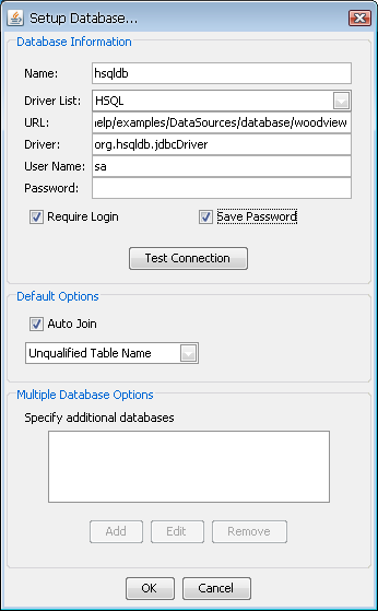
Add Database Dialog
In order for EspressChart to create a connection to the database, the following information must be provided:
- URL:
This JDBC URL specifies the location of the database to be used. A standard JDBC URL has three parts, which are separated by colons:
jdbc:<subprotocol>:<subname>
The three parts of a JDBC URL are broken down as follows:
jdbc- the protocol. The protocol in a JDBC URL is alwaysjdbc.<subprotocol>- the name of the driver or the name of a database connectivity mechanism, which may be supported by one or more drivers. A prominent example of a subprotocol name isodbc, which has been reserved for URLs that specify ODBC data source names. For example, to access a database through a JDBC-ODBC bridge, you have to use a following URL:jdbc:odbc:Northwind
In this example, the subprotocol is
odbcand the subnameNorthwindis a local ODBC data source, i.e.Northwindis specified as a system DSN under ODBC.<subname>- a way to identify the database. The subname can vary, depending on the subprotocol, and it can have a subsubname with any internal syntax the driver writer chooses. The function of a subname is to give enough information to locate the database. In the previous example,Northwindis enough because ODBC provides the remainder of the information.
Databases on a remote machine require additional information to be connected to. For example, if a database is to be accessed over your company Intranet, the network address should be included in the JDBC URL as part of the subname and should follow the standard URL naming convention of
//hostname:port/subsubname
Assuming you use a protocol called
VPNfor connecting to a machine on your company Intranet, the JDBC URL you need to use can look like this:jdbc:vpn://dbserver:791/sales (similar to
jdbc:dbvendorname://machineName/SchemaName)It is important to remember that JDBC connects to a database driver, not the database itself. The JDBC URL that identifies the particular driver is determined by the database driver vendor. Usually, your database vendor also provides you with the appropriate drivers. It is highly recommended that users contact their database driver vendor for the correct JDBC URL that is needed to connect to the database driver.
- Driver:
This is the appropriate JDBC driver that is required to connect to the database. If you are using the JVM included within the installation (or Oracle's J2SE), use the following driver specification to connect to an ODBC data source:
sun.jdbc.odbc.JdbcOdbcDriver
You can also specify a JDBC driver name specific to your database if you are NOT using the JDBC-ODBC bridge. For example, the Oracle database engine will require
oracle.jdbc.driver.OracleDriver.- User Name:
This is the login used for the database.
- Password:
Password for the above user.
Once you specify the connection information, you can test the database connection by clicking the Test Connection button. This will test the connection using the information you've provided and report any problems.
The Default Options portion of the dialog allows you to specify some properties for queries generated through the Query Builder interface or data views. You can specify whether to auto-join selected tables. Auto-join will attempt to join primary and foreign keys defined in the database. You can specify the table name format that should be used for queries either unqualified (only table name), or 2-part or 3-part qualified. Properties specified here will become the default setting for new queries and data views. They can also be modified for individual queries.
The Multiple Database Options portion of the dialog allows you to specify additional databases (i.e. additional database URLs) to obtain data from within the query. This option is only available when the database (original and any additional database) is MS SQL Server and 3-Part Qualified Table Name option is chosen. Note that the same login details as well as the same driver (as defined in the original connection) are used to connect to the specified additional databases as well. The query can obtain data by referencing a column in the additional database using a 3-Part table nomenclature.
There are two sample databases included within the EspressChart installation. One is a HSQL (a pure Java application database) database and the other one is a MS Access database. Both contain the same data and are located in help/examples/DataSources/database directory. For details about how to set up connections to these sample databases, please see Section Q.3 - Set up Data Sources in the Registry.
In addition to connecting to databases via JDBC, EspressChart lets you use the JNDI (Java Naming and Directory Interface) to connect to data sources. In EspressChart, JNDI data sources are treated just like database data sources and support the same functionality (queries, parameters, data views, etc.). The advantage of using a JNDI data source is that it potentially makes it easier to migrate charts between environments. If data sources in both environments are set up with the same lookup name, charts can be migrated without any changes.
To connect to a JNDI data source in the EspressChart, you must have a data source deployed in your Web application environment and you must have EspressManager running as a servlet in the same environment. For more information about running EspressManager as a servlet, see Section 2.3.1 - Starting EspressManager as a Servlet.
To setup a JNDI data source, select the JNDIDataSources node in the Data Source Manager and click the button. This will bring up a dialog allowing you to specify the connection information.
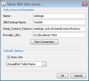
JNDI Setup Dialog
The first option allows you to specify a display name for the data source. The second option allows you to specify the JNDI lookup name for the data source. The third option allows you to specify the initial context factory for the data source, and the last option allows you to specify the provider URL. This information will vary depending on the application server you're using as different vendors implement JNDI data sources differently. You can test the connection by clicking the button.
Once you add a database, a new node for your database will appear in the Data Source Manager window. When you expand the node, you will see two more nodes, one called Queries and one called Data Views. These are the two ways to retrieve data from your database. To create a new query, select the Queries node and click the button. A dialog will come up prompting you to specify a query name and select whether you would like to enter SQL statement or launch the Query Builder.
If you select to enter an SQL statement, a dialog box will come up allowing you to type in your SQL statement. From this dialog, you can also load a QRY or text file containing SQL text, or execute a stored procedure. If you select to launch the Query Builder, the Query Builder will open in a new window, allowing you to construct the query visually. After you finish building or entering the query, you will return to the Data Source Manager window and the query will appear as a new entry under the Queries node for your database.
The Query Builder is an integrated utility that allows you to construct queries against relational databases in a visual environment. To launch the query builder, add a new query within the Data Source Manager and select the Open Query Builder option. The Query Builder will then open in a new window. You can also launch the query builder to modify an existing query by double clicking the query name in the Data Source Manager.
The main Query Builder window consists of two parts. The top half of the window contains all the database tables selected for the queries and their associated columns. The top window also shows what joins have been set up between column fields. The lower half of the main window or QBE (query by example) window contains columns that have been selected or built for the query and their associated conditions.
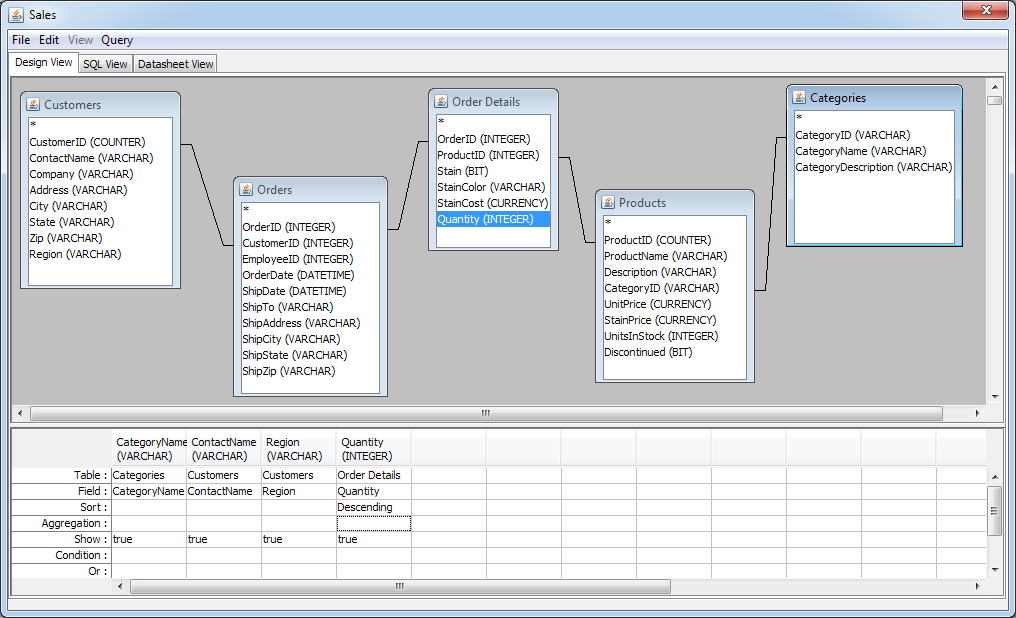
Query Builder Window
There are three tabs at the top of the Query Builder window. These allow you to toggle between different views. The Design View tab is the main designer window described above, the SQL View tab shows the SQL statement that is generated by the current query and the Datasheet View tab shows the query result.
When you finish constructing the query, select Done from the File menu to return to the Data Source Manager.
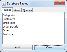
When the Query Builder launches for the first time, a tabbed window will appear containing a list of all the tables within the database. A second tab contains a list of all the views in the database, and the third tab contains a list of other queries you have designed for the database under a heading called Queries. From this window, you can select the tables/views/queries from which you would like to build the query. You can also load a previously designed query as a table. To add a table, select it and click the button or double click on the table name. When a table is added, it will appear in the main Query Builder window and will display all columns within that table. To remove a table, right click within the table and select Delete from the pop-up menu. You can also specify a table alias and sort the fields alphabetically from this menu. You can close the tables window by clicking the button. To re-open it, select Show Tables from the Query menu.
![[Note]](../../../images/note.png) | Note |
|---|---|
By default, the tables will appear using the name format you specified when setting up the database connection. You can change the naming by selecting Table Name Format from the Query menu. |
Query Builder Tables Window
When you select database tables for the query, the Query Builder can auto-detect joins between column fields based on primary key-foreign key relationships in the database. Auto-joins will be added depending on which option you selected when setting up the database connection. Auto-joins will create a standard join between tables. A join is represented by a line drawn between two fields in the top half of the design window. To remove a join or edit its properties, right click on the line and select your choice from the pop-up menu. To add a join, click and drag one column field to another in a different table. A join will then appear. You can change the auto-join settings by selecting Auto Join from the Query menu.
- Join Properties:
Selecting Join Properties from the pop-up menu will bring up three options allowing you to select the type of join used between the column fields. Query Builder only supports equi-joins. Inequality joins can be easily accomplished using the conditions field. You can specify inner joins, left outer joins, and right outer joins. See the examples below for an explanation of the different join types.
Suppose you have the following two tables: Customers and Orders
| CustomerID | CustomerName |
|---|---|
| 1 | Bob |
| 2 | Ivan |
| 3 | Sarah |
| 4 | Randy |
| 5 | Jennifer |
| OrderID | CustomerID | Sales |
|---|---|---|
| 1 | 4 | $2,224 |
| 2 | 3 | $1,224 |
| 3 | 4 | $3,115 |
| 4 | 2 | $1,221 |
An inner join on CustomerID on the two tables will result in combining rows from the Customers and Orders tables in such a way that each row from the Customers table will be “joined” with all the rows in the Orders table with the matching CustomerID value. Rows from the Customers table with no matching CustomerID fields from the Orders table will not be included in the query result set.
Now suppose you create a query by selecting the OrderID, CustomerName, and Sales fields with an inner join on the CustomerID field. The select statement generated by the Query Builder would look like this:
Select Orders.OrderID, Customers.CustomerName, Orders.Sales
From Customers, Orders
Where Customers.CustomerID = Orders.CustomerID
Order by Orders.OrderID;
The result of the query is shown below:
| OrderID | CustomerName | Sales |
|---|---|---|
| 1 | Randy | $2,224 |
| 2 | Sarah | $1,224 |
| 3 | Randy | $3,115 |
| 4 | Ivan | $1,221 |
As you can see, the CustomerName entries “Bob” and “Jennifer” do not appear in the result set. This is because neither customer has placed an order. There are situations where you may want to include all the records (in this example customer names) regardless whether matching records exist in the related tables(s) (in this case the Orders table). You can achieve this result using outer joins.
The Query Builder gives you the option of either right or left outer joins. The keywords “right” and “left” are not significant. It is determined by the order that the tables are selected in the Query Builder. If the outer table (the one that will have all records included regardless of matching join condition) is selected first, then Query Builder will use a right outer join. If the outer table is selected after the other join table, a left outer join is used. In our example, the Customers table has been selected before the Orders table, hence to select all of the records from the CustomerName field, the Query Builder will use a right outer join on the CustomerID fields.
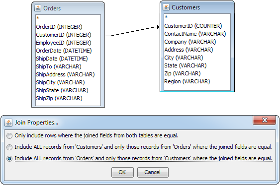
Join Properties Dialog
Now, using the previous example, suppose you create the same query as before, except this time you specify to include all records from the Customers table. The select statement generated by the Query Builder would look like this:
Select Orders.OrderID, Customers.CustomerName, Orders.Sales
From Orders right outer join Customers on Orders.CustomerID = Customers.CustomerID
Order by Orders.OrderID;
The result of the new query is shown below:
| OrderID | CustomerName | Sales |
|---|---|---|
| Jennifer | ||
| Bob | ||
| 1 | Randy | $2,224 |
| 2 | Sarah | $1,224 |
| 3 | Randy | $3,115 |
| 4 | Ivan | $1,221 |
As you can see, all of the customer names have now been selected and null values have been inserted into the result set where there are no corresponding records. If you specify an outer join, the join line connecting the two tables in the Query Builder will become an arrow in the direction of the join.
The QBE window contains information on column fields selected for the query, as well as any conditions for the selection.
- Selecting Column Fields:
You can add column fields to the query from any table that has been selected in one of two ways. You can double-click on a field name within a table to add it to the query, or you can double-click on the Table or Field fields to bring up a drop-down menu with field choices. You can remove a column from the query by right clicking in the lower window and selecting Delete Column from the pop-up menu, or by selecting → . Once you select a column field, you can specify how you want to sort the column, in ascending or descending order, by double clicking on the Sort field. You can also specify group by or column aggregation by double clicking on the Aggregation field. Aggregation options include: Group By, Sum, Average, Min, Max, Count, Standard Deviation, Variance, First, Last, and Where. If you select group by for one column, then you are required to specify group by (or aggregation) for all of the other columns. To specify a column alias, right click on the column and select Alias from the pop-up menu.
- Building Columns:
To build your own column, right click on a blank column in the QBE window and select Build from the pop-up menu. This will launch the Formula Builder. The Formula Builder allows you to construct columns in a visual environment using the tables that you have selected and the formula library for the database that you are using.
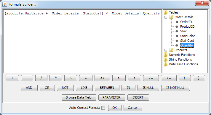
Formula Builder Window
- Conditions:
You can place conditions on the query selection by entering them in the Condition or Or fields. A condition placed in the Condition field creates an
ANDclause within the generated SQL. A condition placed in the Or field creates anORclause within the SQL. Right clicking in either field and selecting Build from the pop-up menu will bring up the Formula Builder. In the Formula Builder, you can specify standard conditions,=, <, >, BETWEEN, LIKE, NOT,etc., as well as construct formulas to filter the query. You can also specify a query parameter here.Note EspressChart can auto-correct items entered as query conditions by appropriately appending the field name and encasing string arguments in quotes. For example, if you enter
= ARC, EspressChart will change the query condition toCategories.CategoryName='ARC'. If you're using complex functions (i.e. database functions that take multiple string arguments), EspressChart may not be able to properly parse the function. You can turn off the auto-correct feature by un-checking the box at the bottom of the formula builder window.
The formula builder component in the query builder allows you to use database specific functions when building a column or condition for the query. You can use the functions that are supplied or add your own to the interface.
EspressChart comes with the function libraries for Oracle, Access, MS SQL, and DB2 pre-loaded. They are stored in XML format in DatabaseFunctions.xml file in userdb directory. For databases with functions not stored in XML, EspressChart will use default ones. You can specify different database functions by editing the XML file or creating a new one based on DatabaseFunctions.dtd file in userdb directory. A sample database functions file might look like this:
<DatabaseFunctions>
      <Database ProductName="ACCESS">
            <FunctionSet Name="Numeric Functions">
                  <Function>Abs(number)</Function>
                  <Function>Atn(number)</Function>
            </FunctionSet>
      </Database>
</DatabaseFunctions>
Sometimes it is necessary to add extra SQL statements to run before or after a query. For example, you may need to set a transaction level or call a stored procedure before executing a query and/or commit a transaction or drop a temporary table after executing a query. The query builder allows you to specify these extra SQL statements by selecting Extra SQL from the Query menu. This will bring up a window allowing you to write statements to execute before and/or after a query.
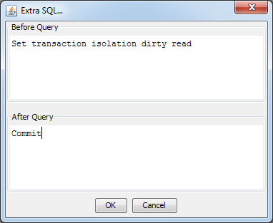
Extra SQL Dialog
You can enter any SQL statements you would like to run before and/or after the query in the appropriate boxes. Once you finish, click the button and the statements will be added to the query.
The SQL View and Datasheet View tabs allow you to see two different views of the query.
- SQL View:
The SQL View tab shows you the SQL statement generated by the query in the design view. It allows you to see how the Query Builder is translating different operations into SQL. You can edit the generated SQL if you want, however, if you change the SQL and then return to the Design View, all changes you made will be lost. If you save a query after changing the SQL, the query will re-open in the SQL View tab if you select to edit it.
- Datasheet View:
The Datasheet View tab shows you the query result in data table form (this tab is also available in the Enter SQL dialog). The datasheet view will show you all the data that is drawn as a result of executing the query. Going to the datasheet view will also test the query to check for design errors. You can navigate the query result by using the toolbar at the bottom of the window.
 Go to the first page of the data table
 Go to the previous page of the data table
 Go to a specific row of data
 Go to the next page of the data table
 Go to the last page of the data table
 Set number of rows to display per page (default is 30)
- Exporting Queries:
You can export queries in one of two ways. You can output the SQL statement as a text or you can output the query result as CSV file. To export a query, select Export from the File menu. A second menu will appear giving you the option to Generate SQL or Generate CSV. Select the desired option and a dialog box will appear prompting you to specify the filename and location.
| Note |
|---|---|
To save the query and exit the Query Builder, select Done from the File menu. |
You can also use the Query Builder to design parameterized queries. This feature allows you to filter the data at run-time. Parameterized queries are also used for parameter drill-down in charts. For more information about drill-down charts, please see Section 7.3 - Parameter Drill-Down.
Query parameters can be defined when typing an SQL statement or using the Query Builder. They can also be defined when running data views (this is covered in the next section). A parameter is specified within an SQL statement by the ":" character. Generally, the parameter is placed in the WHERE clause of an SQL Select statement. For example, the following SQL statement
Select * From Products Where ProductName = :Name
specifies a parameter called Name. You can then enter a product name at run-time and only retrieve data for that product.
Within the Query Builder, you can specify a query parameter by right clicking on the Condition field and selecting Build from the pop-up menu. The Formula Builder will open, allowing you to place a condition on the column.
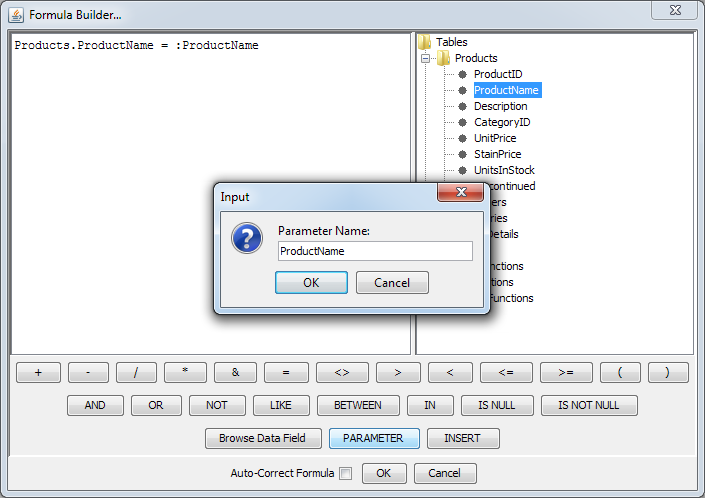
Specifying a Parameter in the Formula Builder
You can insert a parameter by clicking the button. A second dialog will appear prompting you to specify a name for the parameter. Type the parameter name, click and then click again to close the formula builder. You can specify as many different parameters for query as you like.
EspressChart supports a special kind of parameter that takes an array of values as input rather than a single value. Multi-value parameters are useful when you want to filter the result set based on an unknown number of values. For example, say a chart is run to return a list of customers for a specific state/province. Users could select as many different states/provinces as they wanted and return the relevant information.
To create a multi-value parameter, place a parameter within an IN clause in an SQL statement. For example, the following query
Select Customers.Company, Customers.Address, Customers.City, Customers.State, Customers.Zip
From Customers
Where Customers.State IN (:State);
will create a multi-value parameter named State. Multi-value parameters will only be created if there is only one parameter in the IN clause. If you place more than one parameter in the IN clause, i.e. Customers.State IN (:State1, :State2, :State3), it will create three single value parameters instead.
When you attempt to save (by selecting Done from the File menu) or preview (by clicking the Datasheet View tab) a parameterized query, you will first be prompted to initialize the parameter. You can also initialize it by selecting Initialize Parameters... from the Query menu or by clicking the button in the Enter SQL Dialog.
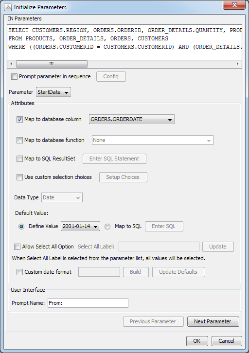
Initialize Parameter Dialog
From this dialog you can specify the following options:
- Map to database column:
This option allows you to specify a column from the database whose values will be used for the parameter input. Selecting this option modifies the parameter prompt that the end user will get when previewing or running the chart in the chart Viewer. If you map the parameter to a database column, then the user will be prompted with a drop-down list of distinct values from which to select a parameter value. If you do not map, the user will have to type in a specific parameter value.
![[Tip]](../../../images/tip.png)
Tip Normally, this drop-down list is populated by running a select distinct on the column while applying the joins and conditions from the query. If you prefer to get all data from the column without constraints (sometimes this can improve performance of the parameter prompts), you can set the
-singleTableForDistinctParamValueargument when starting EspressManager. For more information about EspressManager configuration options, see Section 2.3 - Starting EspressManager- Map to database function:
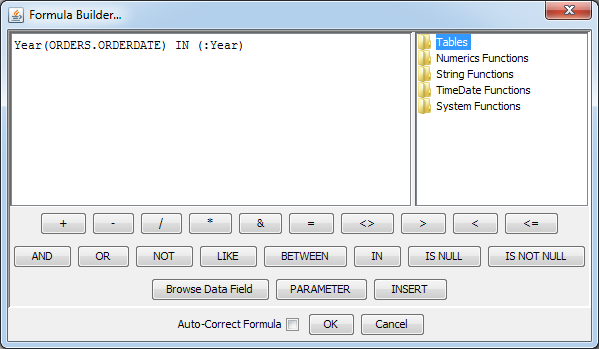
The map to database column feature is very handy if you want to enter a valid value for a parameter from a list box, but sometimes you rather want a computed value or a derived value from a database column. For example, you want to find all orders from year 2007. However, OrderDate is a date. What you want is to apply the Year function to the OrderDate column. This is the impetus behind this feature. Mapping a parameter to a database function is very similar to mapping to a column. In the formula builder, enter a condition comparing a function result to a parameter as shown below:
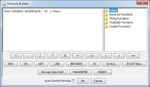
Condition for Mapping to Database Function
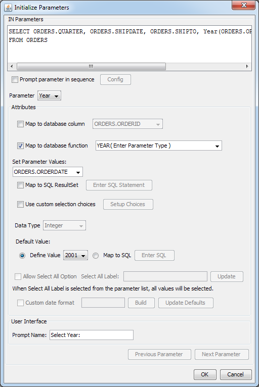
In the initialize parameter dialog, check the Map to database function checkbox and the values will be automatically filled in.
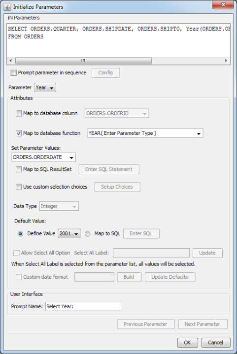
Map Parameter to Database Function
The list of custom functions is extracted from
DatabaseFunctions.xmlfile located in/userdb/directory. Modify the .xml file if you wish to add a new database or custom functions. The new functions will appear in this list after you restart the program.If your database is not listed in the
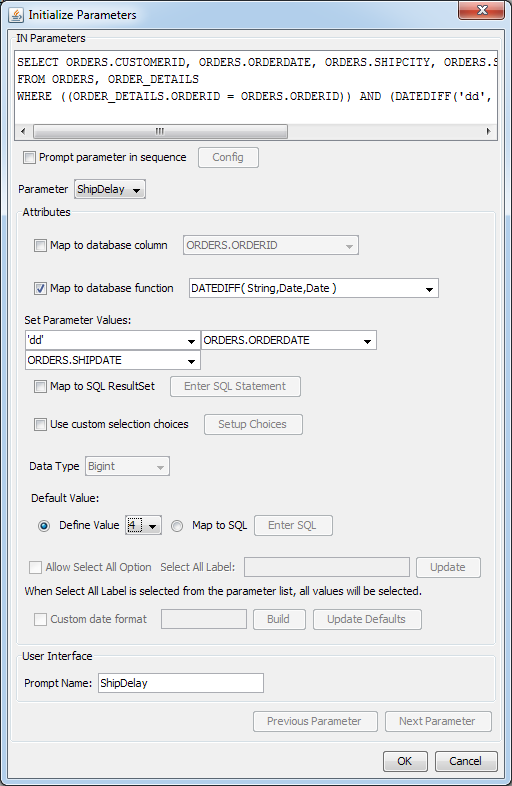
.xmlfile, the function list will be populated with functions listed in the JDBC driver. However, the function parameters are not provided. For example, the HSQL database will not be listed in the.xmlfile.An interesting example using the HSQL database is as follows. Suppose you would like to create a report for orders that were delayed. You can utilize the HSQL DateDiff function to find the number of days for the order to ship.
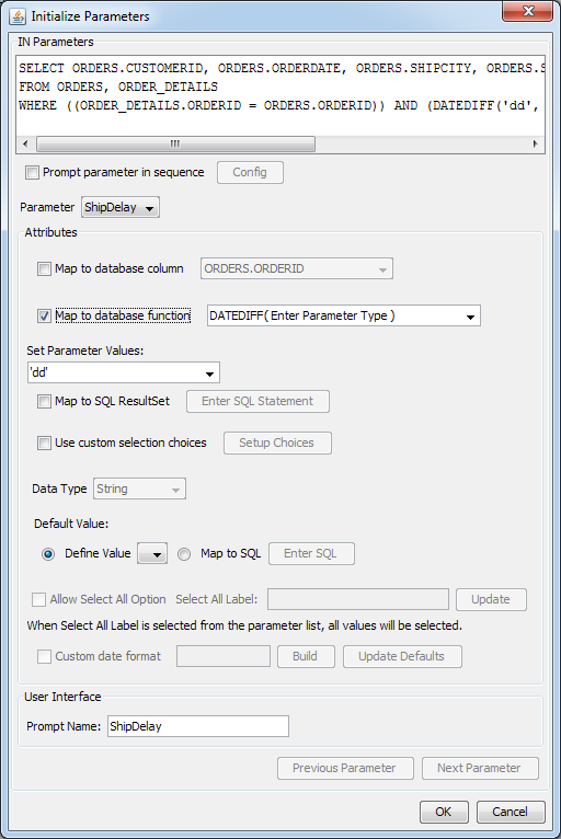
DATEDIFF('dd', ORDERS.ORDERDATE, ORDERS.SHIPDATE) >= :ShipDelayThis function finds the difference between the order date and the ship date and displays the result in terms of days. If you initialize the parameter and check the map to database function, the following window will be displayed:
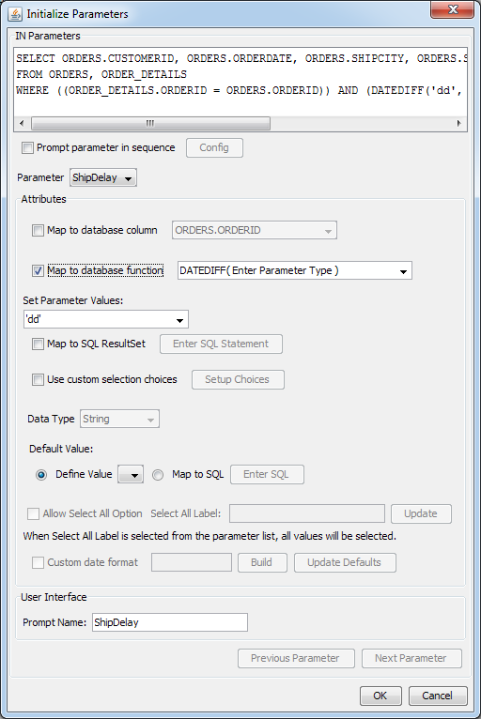
No Parameter Types for HSQL Function
The
DateDifffunction requires a string and two date values for the parameters. Enter these parameter types in the parentheses. This will bring up three set parameter value lists. Enterdd(day) for the first parameter, selectOrders.OrderDatefrom the list for the second parameter, and selectOrders.ShipDatefrom the list for the third parameter. The default values will be updated with the function results.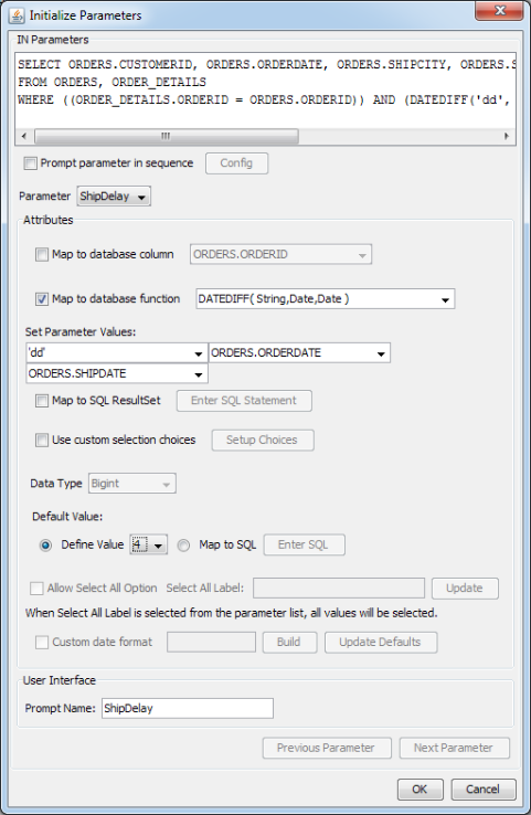
Map Parameter to HSQL Function
- Map to SQL ResultSet:
A parameter mapped to a database column will give you a list of distinct values in a drop-down list box for the user to choose from when running the chart. However, to produce the list of values, a select distinct on the column with the joins and conditions from the query will be run. In some cases, this can be a time-consuming process. To obviate this problem, and in fact gain complete control as to what and how to populate the drop-down list box, you can write your own select statement to populate the drop-down list. An added bonus is that parameters that are in the query can be included in this query. With proper joins and parameters included, you can use this feature to facilitate cascading parameters. An example is as follows:
Suppose you have two parameters in the query. So, your query is as follows:
SELECT CATEGORIES.CATEGORYID, PRODUCTS.PRODUCTNAME, PRODUCTS.UNITPRICE, PRODUCTS.UNITSINSTOCK
FROM PRODUCTS, CATEGORIES
WHERE ((PRODUCTS.CATEGORYID = CATEGORIES.CATEGORYID))
AND (((CATEGORIES.CATEGORYID =:category) AND (PRODUCTS.PRODUCTNAME =:product)))
In the
configprompt ininitialize parameter, set the order for parameter prompting tocategoryfirst, thenproduct.The select statement for parameter
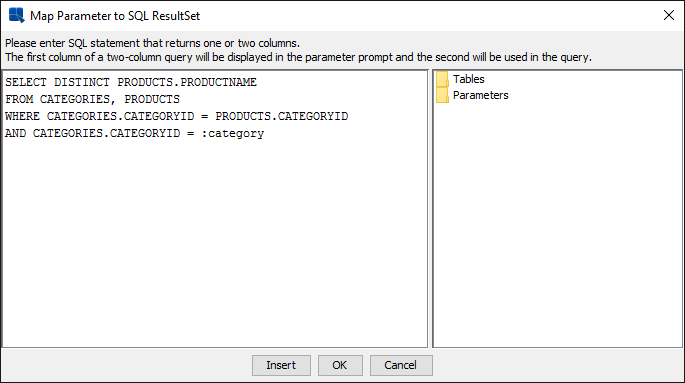
categorycan be the following:SELECT DISTINCT CATEGORIES.CATEGORYID FROM CATEGORIESThe select statement for parameter
productwill be as shown below:SELECT DISTINCT PRODUCTS.PRODUCTNAME FROM CATEGORIES, PRODUCTS WHERE CATEGORIES.CATEGORYID = PRODUCTS.CATEGORYID AND CATEGORIES.CATEGORYID = :category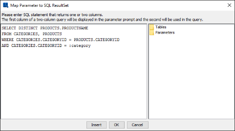
Select Statement for Product
When the user runs the template,
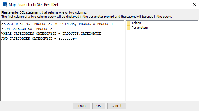
categorywill be prompted first. Then the value ofcategorychosen will be used to filter forproduct.The select statement mapped to a parameter can have either one or two columns in the select list. It is clear that if one column is in the select list, it must be the column that supplies list of distinct values for the parameter. Another useful feature provided here is that you can actually select two columns in the select list such that the first one of the columns will supply values for the drop-down list while the second column will be the actual parameter value for the filter condition. Consider the following example.
Suppose your database has a table with product ID as the primary key. When your end user wants to search for products from the database, they want to use the product name as parameter (therefore it is listed in the query as first) since a product ID could be just a cryptic code (therefore it is listed in the query as second). Using this feature, you can choose product name for the values in the drop-down list and product ID as the actual value filter condition.
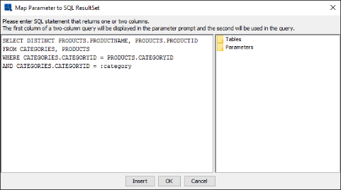
Select Statement with Two Columns
- Use custom selection choices:
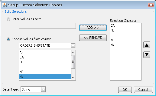
Rather than having a drop-down menu with all the distinct column values, you can also create a custom list of parameter values. To create this list, select this option and click the button. This will launch a new dialog allowing you to create a list of choices.

Custom Parameter List Dialog
In this dialog, you can either enter custom values or select values from the distinct values of a column in the database. Once you finish specifying the values for the list, click the button and the choices will be saved.
- Default Value:
This allows you to specify a default value for the parameter. Although you don't have to specify a default value, it is recommended that you do so. If you do not supply a default value, you cannot open or manipulate the chart template without the data source present.
You can either select a single value manually (either choose it from a list or type it manually, it depends on the mapping method you chose) or map the default value to a SQL query.
For multi-value parameters (see Section 4.2.2.2.1 - Multi-Value Parameters), the SQL query can return more than one value. In such case, several values will be chosen as default parameter values.
- Date Variable:
This option is only available when the parameter is not mapped to a database column or function, or it's mapped to a SQL resultset and not set to a custom selection choice. This option is only intended for parameters with variable type date/time. When you click this button, the following panel will pop up, listing all the supported keywords.
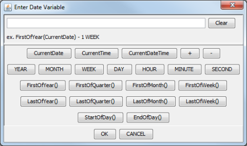
Enter Date Variable Dialog
This dialog allows you to select one of the three keywords:
CurrentDate,CurrentTime, andCurrentDateTime. You can add or subtract units of time from the current date/time, allowing you to have a dynamic date range. For example, a chart can have the following default values:StartDate: CurrentDate - 1 WEEK EndDate: CurrentDateThis would indicate that every time the chart is run, the default prompt should be one week ago to the current date. Other supported time units are
YEAR, MONTH, DAY, HOUR, MINUTE, andSECOND. This feature only supports a single addition or subtraction, it does not support multi-value parameters.You can also use functions to define the parameter value:
- FirstOfYear()
Argument format:
CurrentDate,CurrentDateTime, e.g.FirstOfYear(CurrentDate)This function returns a date of the first day of the year from the argument. For example, when the argument evaluates to
2012-08-14, the function returns2012-01-01.- LastOfYear()
Argument format:
CurrentDate,CurrentDateTime, e.g.LastOfYear(CurrentDate)This function returns a date of the last day of the year from the argument. For example, when the argument evaluates to
2012-08-14, the function returns2012-12-31.- FirstOfQuarter()
Argument format:
CurrentDate,CurrentDateTime, e.g.FirstOfQuarter(CurrentDate)This function returns a date of the first day of the quarter which includes the date from the argument. For example, when the argument evaluates to
2012-08-14, the function returns2012-07-01.- LastOfQuarter()
Argument format:
CurrentDate,CurrentDateTime, e.g.LastOfQuarter(CurrentDate)This function returns a date of the last day of the quarter which includes the date from the argument. For example, when the argument evaluates to
2012-08-14, the function returns2012-09-30.- FirstOfMonth()
Argument format:
CurrentDate,CurrentDateTime, e.g.FirstOfMonth(CurrentDate)This function returns a date of the first day of the month from the argument. For example, when the argument evaluates to
2012-08-14, the function returns2012-08-01.- LastOfMonth()
Argument format:
CurrentDate,CurrentDateTime, e.g.LastOfMonth(CurrentDate)This function returns a date of the last day of the month from the argument. For example, when the argument evaluates to
2012-08-14, the function returns2012-08-31.- FirstOfWeek()
Argument format:
CurrentDate,CurrentDateTime, e.g.FirstOfWeek(CurrentDate)This function returns a date of the first day of the week which includes the date from the argument. For example, when the argument evaluates to
2012-08-14, the function returns2012-08-12(Sunday is considered as the beginning of the week).- LastOfWeek()
Argument format:
CurrentDate,CurrentDateTime, e.g.LastOfWeek(CurrentDate)This function returns a date of the last day of the week which includes the date from the argument. For example, when the argument evaluates to
2012-08-14, the function returns2012-08-18(Saturday is considered as the end of the week).- StartOfDay()
Argument format:
CurrentTime,CurrentDateTime, e.g.StartOfDay(CurrentDateTime)This function returns a time of the start of the day from the argument. For example, when the argument evaluates to
2012-08-14 12:15:03, the function returns2012-08-14 00:00:00.0.- EndOfDay()
Argument format:
CurrentTime,CurrentDateTime, e.g.EndOfDay(CurrentDateTime)This function returns a time of the end of the day from the argument. For example, when the argument evaluates to
2012-08-14 12:15:03, the function returns2012-08-14 23:59:59:999.
- Data Type:
This allows you to specify data type for the parameter value(s). If you mapped the parameter to a column, the data type is set automatically.
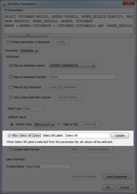
- Allow Select All Option:
Use this to add an option to the parameter prompt dialog that will allow users to select all parameter values even for single-value parameters. See the Section 4.2.2.2.3 - All Parameters for more details.
- Custom Date Format:
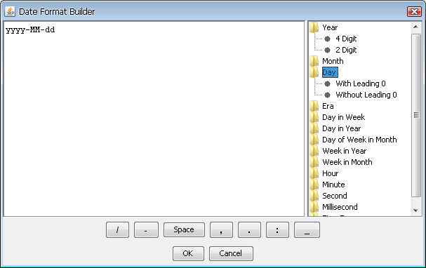
This allows you to set the format in which the date parameter should be entered. This option is only available if you have not mapped the parameter to a column or entered custom selection choices (i.e. the end user will be typing in the date value). When you check this option, you can enter the date format in a combination of characters that represent time elements. You can build the format easily using the date format builder by clicking the button.
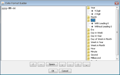
Date/Time Format Builder
The builder contains a list of elements available on the right. You can mouse over the elements to see an example of each presentation. The bottom section contains a set of separators available for use.
The following table illustrates the character combinations that you can use:
Character Represents Output(text/number) Example G era text AD y year number 1996, 96 M month in year text or number (depends on length) July, Jul, 07 d day in month number 10 h hour am/pm (1-12) number 1 H hour 24 hr. (0-23) number 18 m minute in hour number 30 s second in minute number 55 S milisecond number 978 E day in week text Tuesday, Tue D day in year number 189 F day of week in month number 2 (as in 2nd Wed. in July) w week in year number 27 W week in month number 2 a am/pm marker text AM, PM k hour 24 hr (1-24) number 24 K hour am/pm (0-11) number 0 z time zone text Pacific Standard Time, PST You can piece together almost any combination of these characters to produce a date expression in the format you want. The count of groups of characters determines the form the element will take. For text elements, 4 or more characters in a group will cause the full form of the element to be used. If less than 4 characters are used, the short form will be used, if it exists. For example,
EEEEwould returnMondayandEEwould returnMon. For monthMwhich can be displayed as either text or a number, 4 or more in a group will display the full version, 3 will display the abbreviation, and 2 or less will display the number form.For numeric elements, the count of characters is the minimum number of digits that the element will take. Shorter numbers will implement leading zeros. For example, if the day of the date is 2,
ddwould return02anddwould return2.Any character that is not a-z or A-Z like “;”, “:”, “@”, etc. can be inserted anywhere within the string expression and will be displayed as entered. You can also insert words and expressions by enclosing them within single quotes (type two single quotes to insert an apostrophe as text).
- Prompt Name:
This allows you to specify the prompt that is given to the user in the parameter dialog.

If you map the parameter, the user will see either a drop down box (single value parameter) or a list box (multi-value parameter) containing various options. If you choose not to map the parameter, the user will see a textbox to enter their own value. In case of a multi-value parameter, it is recommended to let the user inform in the parameter prompt that this parameter accepts multiple values. Users can separate multiple values using a comma (e.g. ARC, DOD, TRD). If the text requires the use of comma, the user can use quotes to include the comma within the filter string (e.g. "Doe, John", "Smith, Mike").
Clicking the and the buttons allows you to initialize each of the parameters that have been defined in the query.
When you select to use a parameterized query to design a chart, or open a chart that uses a parameterized query, the chart will load/start with the default values. You will be prompted to provide parameter values when you preview the chart.
Sometimes you want to select all parameter values at once. The All Parameters feature allows you to do so.
- Single-value parameters
It is possible to select all parameter values at once, even for parameters that do not allow multi-value selection.
Note There is a difference between multi-value selection and all-value selection. See the Inner Workings chapter to learn more.
For example: Let's assume you have a condition like this:
WHERE column = :ParameterIn such case, the parameter prompt dialog will not allow you to select more than one value.
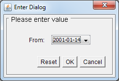
Typical single-value parameter
But you can use the Select All Values feature to add an option to the parameter value list that will allow viewers to select all parameter values at once (even if the parameter does not allow multi-value selection).
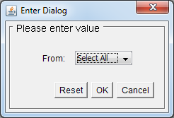
Single-value parameter with the Select All functions enabled
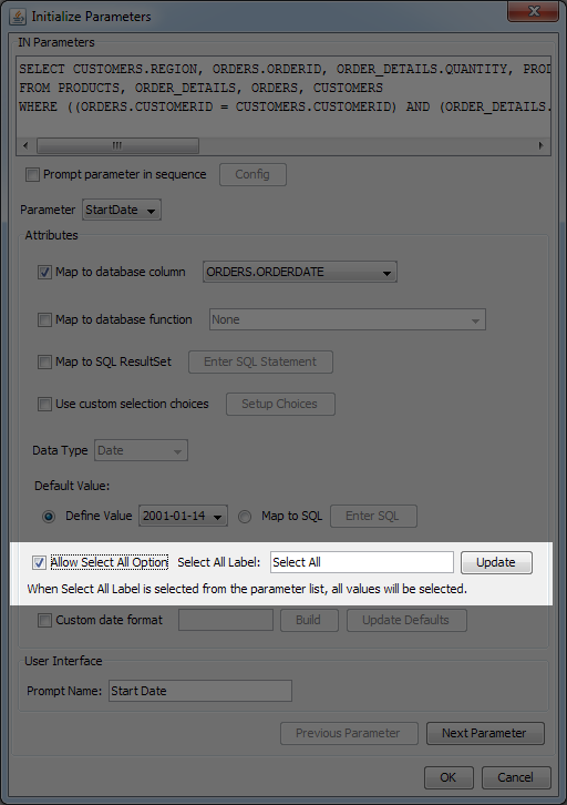
The Select all feature can be enabled in the Initialize Parameters dialog (see Section 4.2.2.2.2 - Initializing Query Parameters for more details) by selecting the Allow Select All Option checkbox.
This option is only available for parameters that meet the following requirements:
The parameter uses one of the following operators. If there are multiple occurrences of this parameter in the query, all parameter comparison operators have to be one of these:
<
less than
<=
less than or equal to
>
greater than
>=
greater than or equal to
=
equal to
The parameter is mapped to the same column as the column from the parameter condition or the parameter isn't mapped to anything.
After you select the Allow Select All option, the Select All Label field activates, allowing you to enter a text that will be used for selecting all data from the query. For parameters that are mapped to a column, this text will be displayed in the parameter value list in 1st place. For parameters that aren't mapped to anything, entering this text as the parameter value will result in selecting all data.
- Multi-value parameters
Unlike single-value parameters, the Select All feature is enabled for all multi-value parameters by default (in fact, it can't be disabled, because disabling it for multi-value parameters would make no sense). All you have to do to use this feature is to click on the
 Select All icon in the parameter prompt.
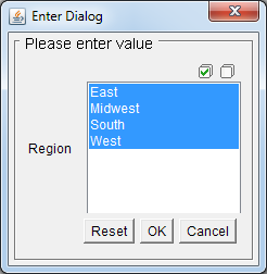
However, multi-value parameters can work in two modes:
If the parameter meets the conditions from the previous paragraph and the parameter is on the first cascading level (i.e. parameter cascading is disabled or the parameter is on the first cascading level), it is parsed by the SQL parser and the parameter condition is nullified. Nullifying the parameter optimizes the query and prevents it from causing performance issues or even errors. See the Inner Workings to learn more about how it works.
If the parameter doesn't meet the conditions from the previous paragraph or if it's not on the first cascading level, selected values will be injected to the query as a list of values separated by comma. If there is a large amount of values injected to the query as a list, the query can become quite long. Long queries can cause performance issues or even errors, so it is not recommended to use this option for parameters with many values.
- Inner Workings
If a chart viewer chooses to select all parameter values for a single-value parameter or for a multi-value parameter that meets the conditions for parameter disabling, the query is then automatically parsed and a special condition is added to the parameter which basically disables the parameter.
For example: The following query
select *
from table
where column > parameter_value
Would be parsed and passed to the database as:
select *
from table
where ((column > parameter_value) OR (1 = 1))
This example also demonstrates another important thing: selecting all values for the < (less than) or > (greater than) operators returns all values from the table (if there are no other conditions) rather than returning no data at all (because condition like
WHERE <all data from the Date column> > Datewould return no data...).Because EspressChart allows you to use many database systems, parsing may fail for certain complex queries in certain databases. In such case a warning dialog will be displayed.
In such situations, you have the following three options:
Try to modify the query so it can be parsed by our parser.
Add your own Select all parameters condition to the query.
For example:
WHERE ((column = :Parameter) OR (:Parameter LIKE 'selectall'))Note If you embed all parameters directly to the query, leave the Allow Select All Option option disabled.
Contact Quadbase support.
Typically, the Query Builder is recommended for creating queries. However, there are cases when it is necessary to enter SQL statements directly: for example if the query is already created in a QRY file, if the query is built into a stored procedure/function, or if the query requires commands not supported by the Query Builder. In these situations, select Enter SQL statement to open the Set SQL Statement window. Here you can enter SQL statements directly into the text area as shown below or you can load an existing QRY File.
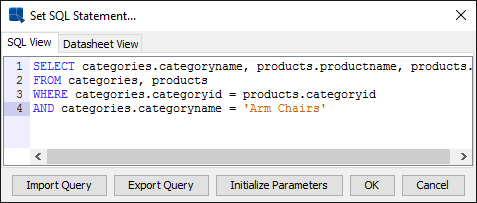
Enter SQL Statement Dialog
To preview the result set, click on the Datasheet View tab.
Compared to other database systems, Oracle uses a different approach when it comes to stored procedures and functions. For example, on MS SQL Server, using the EXEC command will return a result set. However, Oracle requires the use of an OUT parameter with a REF CURSOR type to return the result set. In addition, Oracle will not accept multiple statements from a single query. Therefore, it is necessary to store the query within a stored function and use special syntax to access the existing Oracle stored procedures.
To access your Oracle stored procedures, the first step is to define a weakly typed REF CURSOR using the following PL/SQL statement:
CREATE OR REPLACE PACKAGE types
AS

      TYPE ref_cursor IS REF CURSOR;

END;
This ref_cursor type will be used to store the query result set and return as an OUT parameter. The next step is to create a function which calls your stored procedure and executes your query. The following skeleton code will return a simple query using the ref_cursor type.
CREATE OR REPLACE FUNCTION my_function()

      RETURN types.ref_cursor

AS

      result_cursor types.ref_cursor;

BEGIN

      do_stored_procedure();
      OPEN result_cursor FOR
            SELECT * FROM Categories

      RETURN result_cursor;

END;
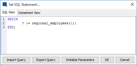
Now that the Oracle stored function is set up, it can be easily called from ChartDesigner using a special PL/SQL like syntax. In the Set SQL Statement window, enter the following syntax to call the Oracle stored function:
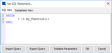
Calling simple Oracle stored function
The BEGIN ... END; syntax alerts the system that the user is trying to access an Oracle stored function. And the “?” notifies the ChartDesigner that a variable is reserved for the OUT parameter. The JDBC syntax for calling Oracle stored procedures is as follows:
( call ? := my_function() )
However, EspressChart does not support this format. Preview the results by clicking the Datasheet View tab.
Here is a more practical example to illustrate how stored procedures can be used with EspressChart to develop useful solutions. Suppose you have a table called employee_table that stores an organization's location hierarchy such as the one shown below:
| ID | NAME | PARENT | EMPLOYEE |
|---|---|---|---|
| 1 | All | NULL | 0 |
| 2 | America | 1 | 0 |
| 3 | Europe | 1 | 0 |
| 4 | New York | 2 | 20 |
| 5 | Santa Clara | 2 | 30 |
| 6 | Dallas | 2 | 12 |
| 7 | London | 3 | 14 |
| 8 | Paris | 3 | 11 |
The table lists various corporate locations in a tree structure. The numbers of employees are stored in the leaf nodes (e.g. New York, London, etc.) and each node contains information about its immediate parent. Suppose you want to create a chart that displays the number of employees in a certain region and information about the separate branches within that region. For example, if the user inputs ID = 2 (America), you want the chart to display the total number of employees in America along with the branch locations. Using Oracle's CONNECT BY and START WITH clauses, the problem can be solved with two simple Oracle Stored Functions:
CREATE OR REPLACE FUNCTION sum_employees(locID IN NUMBER)

      RETURN NUMBER

AS

      sum_emp NUMBER;

BEGIN

      SELECT sum(employee) INTO sum_emp
      FROM employee_table
      CONNECT BY PRIOR id = parent
      START WITH id = locID;

      RETURN sum_emp;

END;

CREATE OR REPLACE FUNCTION regional_employees (locID IN NUMBER)

      RETURN types.ref_cursor

AS

      result_cursor types.ref_cursor;

BEGIN

      OPEN result_cursor FOR
            SELECT id, name, sumEmployees(id) AS Employees
            FROM employee_table
            CONNECT BY prior id = parent
            START WITH id = locID;

      RETURN result_cursor;

END;
The function sum_employees takes the starting node as an argument and finds the sum of all leaf nodes that are descendents of that node. For example, sum_employees(3) returns 25 because there are 25 employees in Europe (14 in London, 11 in Paris). The second function, regional_employees, traverses through the tree structure starting with the locID and builds a result set from the ID, Name and the result from the sum_employees function. The result set is then returned through a REF CURSOR.
To call a stored function that requires an argument, enter the following statements in the Set SQL Statement window:
Calling regional_employees function
Preview the results by clicking the Datasheet View tab.
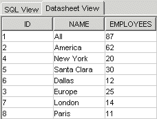
Result set from regional_employees
As seen in the results, the CONNECT BY clause traverses the tree recursively listing the American nodes together before listing the European nodes. If the user is only interested in European locations, they can enter 3 for the parameter and the following result set would return this:
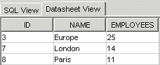
Result set from regional_employees in Europe
To create a parameterized chart, use the :param_name syntax. The SQL parser in EspressChart will be able to differentiate between the colon used for parameters and the one used for the assignment operator (:=). Here is an example of using the parameters:
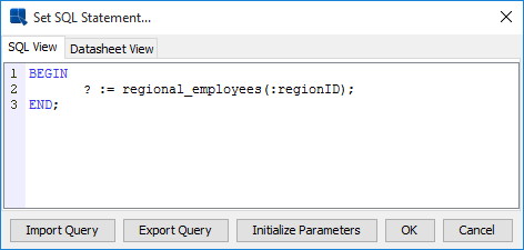
Calling Oracle Stored Function using Parameter
When using IN parameters, it is necessary to initialize the parameters prior to executing the query. It is especially important to set the correct default data type for executing stored procedures, because the parameters cannot be mapped to existing columns. You can find more information about initializing parameters in Section 4.2.2.2.2 - Initializing Query Parameters. To try this example, <EspressChartInstall>\help\examples\data\locationHierarchyExample.sql contains SQL commands to create employee_table as well as two stored functions.
In addition to the query interfaces, EspressChart provides another way of retrieving database data - data views. Data views provide a simplified view of the database in which users can design queries by simply selecting fields without using the Query Builder or having any knowledge of the underlying database structure. Using data views, administrators can predefine tables, joins, and fields, creating a local schema for the user to select from.
For example, an administrator could set up a data view for the sales department. The appropriate database tables and fields are pre-selected and grouped in a manner congruent with business users' logic. For example a group called “invoices” would have the appropriate customer and order fields. End users would then select this data view, pick the pertinent fields, specify a date range, and then begin designing a chart.
To create a data view, select the Data Views node in the Data Source Manager window and click the button. A new window will open allowing you to select the database tables you want to use for the data view.
Data View Choose Tables Dialog
Left window contains all available database tables and views. You can add a table by selecting it in the left window and clicking the button. By default, the data view will use the name format you specified when setting up the database connection. You can change the naming by clicking the button, or specify a table alias by clicking the button. You can also import selected tables and joins from another data view by clicking the button.
The Joins tab of this window allows you to specify the joins between the selected tables.
Data View Joins Dialog
The Joins tab shows all selected tables and their associated fields. The tables will be auto-joined depending on which option you selected when setting up the database connection. These auto-joins create a standard join between tables represented by a line. To remove a join or edit join properties, right click on the line and select your choice from the pop-up menu. To add a join, click and drag one column field to another in a different table. A join will then appear. Data views use the same join properties as the Query Builder. For more information about join properties, please see Section 4.2.2.1.2 - Joins.
After you finish selecting and joining tables, click the button and a new window will open allowing you to construct the data view.
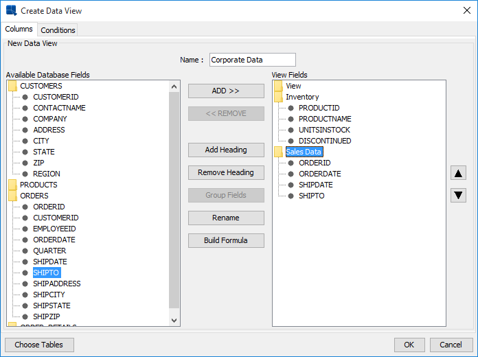
Create Data View Dialog
The left window contains a list of tables you have selected and their associated fields. Each folder represents a table and can be opened and closed by double clicking. The right window contains fields that have been selected for the data view. To add a field to a data view, select it in the left window and click the button. Fields can be removed from the data view in the same way by selecting a field in the right window and clicking the button. You can create a calculated column by clicking the button. This will open the formula builder, allowing you to build the column. You can also define an alias by selecting any of the view fields in the right window and clicking the button.
You can also group fields within the data view by adding headings. This allows you to create your own organizational structure of virtual tables that group data from different database tables under one heading. To create a heading, click the button. You will then be prompted to specify a name for the heading. The new heading will then appear as a folder in the right window. To add fields under a heading, first select the fields you want to add from the right window and click the button. You will then be presented with a drop-down menu, allowing you to select the heading under which you would like to add the fields.
The Conditions tab contains a formula builder window that allows you to specify certain filtering criteria for end users. Anything added in this window will be added to the Where clause of the generated SQL. For more information about using the formula builder, please see Section 4.2.2.1.3 - Columns.
Once you finish creating the data view, click the button and the data view will be added to the Data Source Manager. Users can now use this view to construct ad-hoc queries.
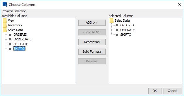
When you design a chart using a data view as the data source (by selecting the data view and clicking the button), a window will open allowing you to select which fields in the view you want to use for the chart. From this dialog, you can also build computed fields based on the available view columns.
After you select the fields, click the button and a new window will open allowing you to specify sorting, aggregation, and filtering conditions for the data view.
Data View Choose Fields Dialog
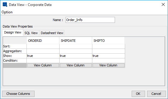
Data View Conditions Window
You can specify sorting, aggregation, and conditions for every field in the data view by double clicking on the respective field. Sorting and aggregation can be selected from drop-down menus. Double clicking on the Conditions field brings up a new window that allows you to specify simple selection criteria like >, <, =, and between. Users can build more advanced filtering criteria by right clicking on the Conditions field and selecting Build from the pop-up menu. This will open the Formula Builder window allowing you to build a condition. You can also display all of the unique values in the column by double clicking on the button.
The Option menu in the upper left corner of the conditions window allows you to select a vertical/horizontal view for the conditions window, initialize any parameters in the data view, or save the query.
The selection set and conditions that you specify will be saved as a data view query with the name that you specify in the name field. Data view queries are saved under the node for the data view. A chart created from the data view will refer to the data view query for updating/modification.
As with Query Builder, users can specify query parameters in Data Views. To add a parameter to a data view, select a data view in the Data Source Manager and click View to run the data view. After you select fields for the data view and you are in the conditions window, right-click in the Condition field for a column and select Build from the pop-up menu. This will bring up the formula builder, allowing you to specify a parameter in the same way as in Query Builder. For more information about this, please see Section 4.2.2.2 - Parameterized Queries.
Once you enter the parameter, you will be prompted to initialize it if you go to the Datasheet View tab and then click to continue with the chart wizard, or if you save the selections as a query. You can also initialize the parameter by selecting Initialize Parameters from the Option menu.
Sometimes you may need to make changes to the structure/make-up of the data view as your data model or requirements change. Changes could include adding/removing fields or re-naming them. You can propagate changes from the data view to its associated queries by selecting it in the data source manager and selecting Data View Queries from the Update menu.
All of the queries associated with the view will be scanned and any inconsistencies in fields or field names will be presented for you to update.
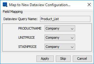
Update Query Fields Dialog
For each query, you will be prompted to change any fields that no longer match the data view structure. For each field, you can select a field from the data view to map it to, or remove the field from the query. If you do not want to change anything in the query, you can click the button. The query will continue to run, but it will refer to the old data view structure. Click the button to save the changes to the data view query.
If you select to build a chart using database data either by designing a query in the Query Builder, writing an SQL statement, or running a data view, you can modify the query directly from the Chart Designer without having to go back to the Data Source Manager.
To modify a chart's query, select Modify Query from the Data menu in Chart Designer. If you have designed a query in the Query Builder, the Query Builder interface will re-open allowing you to modify the query. If you have entered an SQL statement, a textbox will open allowing you to modify the SQL. If you have used a data view, the data view conditions window will re-open allowing you to change the filters or pick additional fields.
Once you specify all the changes, you will be given an option to modify the query in the data registry, save a new query in the data registry, or modify only the query in the template.
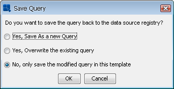
Saving Query Options
Once you specify the save options, the modified query will be applied to the chart. Note that if you made significant changes to the query, you may need to perform the data mapping for the chart again. For more information about data mapping, please see Chapter 5 - Chart Types and Data Mapping.
If you have selected to build a chart using database data, you can also directly edit a template's database connection information from within the chart Designer. To modify the connection information in the chart, select → . This will bring up a dialog allowing you to specify a different setting for the chart to use when connecting to the database or JNDI data source.
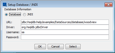
Change Database Connection Dialog
In addition to manually entering the database information, you can retrieve the database connection information from a data registry. To do this, click the button on the Database Connection dialog. This will allow you to browse to XML registry file from which you want to pull the database connection. When you select a registry file, you will be presented with a list of databases defined in the registry.
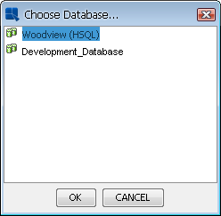
Select Database from Registry
Select the database that you want to use and click the button. The connection information for that database will be automatically applied to the connection dialog. After you set the connection information for the template, click the button and the changes will be applied.
Unlike the modify query feature, changes to a template's database connection will only saved be to the template. It will not be saved to the data registry.